Tutorial 1: Data Preparation

Welcome to tutorial on using the mTopic package to prepare data for multimodal topic modeling of single-cell data. The mTopic package supports spatial and non-spatial multimodal topic modeling, enabling the discovery of complex patterns across multiple modalities in single-cell experiments.

Data preprocessing is a crucial first step in any single-cell analysis workflow. It ensures the data is clean, well-structured, and suitable for downstream modeling. This includes filtering out uninformative features, normalizing raw counts, and aligning modalities for comparability. These steps are essential to produce biologically meaningful and statistically robust topic models.

This tutorial will demonstrate how to preprocess a multimodal dataset in preparation for topic modeling using mTopic.

We use a publicly available dataset from GEO (GSE218593 and GSE205055), which includes ATAC and RNA measurements from P22 mouse brain. A preprocessed .h5mu file version of this dataset is available at Zenodo.

We will begin by downloading the dataset from Zenodo.

! wget -O P22MouseBrainATAC_raw.h5mu \
  "https://zenodo.org/records/20044694/files/P22MouseBrainATAC_raw.h5mu?download=1"

--2026-05-06 21:06:10--  https://zenodo.org/records/20044694/files/P22MouseBrainATAC_raw.h5mu?download=1
Resolving zenodo.org (zenodo.org)... 137.138.153.219, 188.185.48.75, 188.184.103.118, ...
Connecting to zenodo.org (zenodo.org)|137.138.153.219|:443... connected.
HTTP request sent, awaiting response... 200 OK
Length: 80339872 (77M) [application/octet-stream]
Saving to: ‘P22MouseBrainATAC_raw.h5mu’

P22MouseBrainATAC_r 100%[===================>]  76.62M  75.6MB/s    in 1.0s

2026-05-06 21:06:12 (75.6 MB/s) - ‘P22MouseBrainATAC_raw.h5mu’ saved [80339872/80339872]

The mTopic package operates on MuData objects, which organize multimodal single-cell data by combining multiple AnnData layers—each representing a modality such as ATAC, RNA, or protein epitopes into a single structure. These are stored in .h5mu files, an HDF5-based format optimized for efficient access.

In this tutorial, we load a MuData object named mdata, which contains raw ATAC and RNA data from P22 mouse brain.

import mtopic

mdata = mtopic.read.h5mu("P22MouseBrainATAC_raw.h5mu")

mdata

MuData object with n_obs × n_vars = 9215 × 92955
  obsm:     'coords'
  2 modalities
    rna:    9215 x 22803
    atac:   9215 x 70152

Before running topic modeling, the data must be preprocessed to ensure it is clean, informative, and suitable for analysis. The filtering pipeline includes the following steps:

• Permutation of counts (mtopic.pp.permute):

  Randomizes cell counts within each feature to estimate technical noise and identify overrepresented features.
• Transformation of count matrices:

  TF-IDF (mtopic.pp.tfidf) is applied to ATAC, histone modification, or RNA data to highlight informative features.

  CLR normalization (mtopic.pp.clr) is used for protein epitope data to correct compositional bias (here, we skip this normalization step, as we have only ATAC and RNA modalities).
• Scaling counts (mtopic.pp.scale_counts):

  Scales total counts across modalities to ensure equal contribution during modeling.

These steps improve data quality and reduce technical artifacts, enhancing the interpretability of the resulting topics.

mtopic.pp.permute(mdata)
mtopic.pp.tfidf(mdata, mod="atac")
mtopic.pp.tfidf(mdata, mod="rna")
mtopic.pp.scale_counts(mdata)

The data is now ready for an initial round of topic modeling to help identify technical noise and overrepresented features. We recommend training a simple mtopic.tl.MTM model for this step.

If working with a large dataset, consider selecting a representative subset of observations to reduce runtime. For smaller datasets, such as the one used here, which contains 9,215 spatial spots, the filtering model can be trained on the full dataset.

model = mtopic.tl.MTM(mdata, n_topics=10, n_jobs=100)
model.VI(n_iter=30)

100%|██████████| 30/30 [03:21<00:00,  6.72s/it]

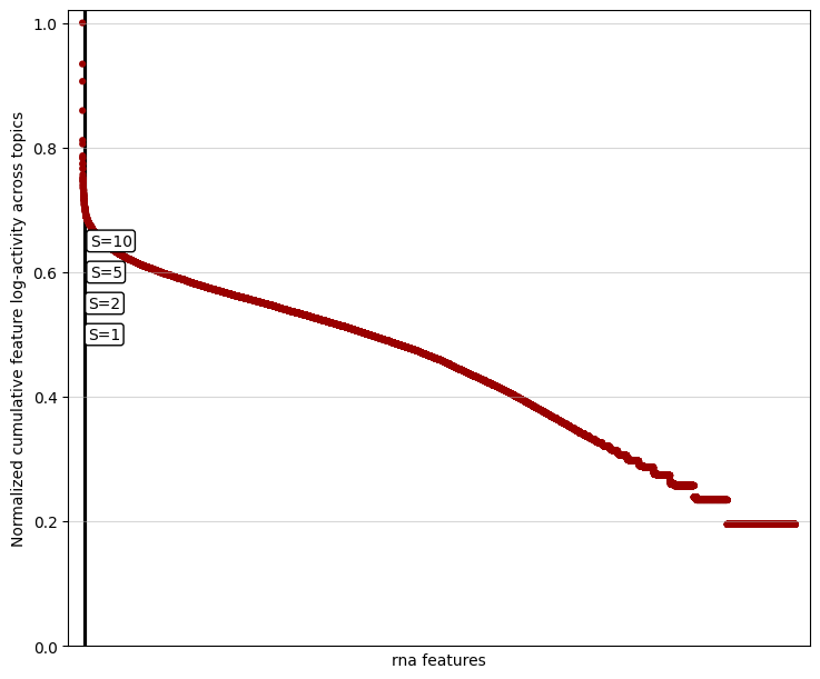
After training the filtering-oriented model, the next step is to identify overrepresented features with disproportionately high cumulative feature scores across all topics. These features often reflect technical noise rather than a meaningful biological signal.

We apply a knee detection algorithm to filter them, which identifies a sharp drop in cumulative feature scores and defines a cutoff point for filtering. The sensitivity of this detection is controlled by the knee_sensitivity parameter (S), which determines how pronounced the drop must be to qualify as a knee. Higher values of S result in more aggressive filtering, while lower values yield more conservative thresholds.

For example, below is a knee plot for the RNA modality, showing the distribution of cumulative feature scores and example detected cutoffs.

mtopic.pl.filter_var_knee(model, mod="rna")

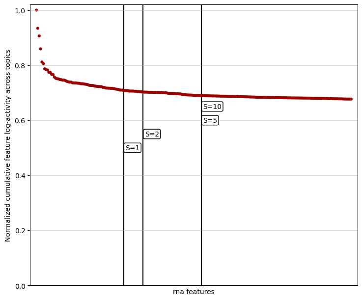
In datasets with many features, the knee point may be challenging to detect due to the dense distribution of values. To improve visibility, you can limit the plot to the top-scoring features by adjusting the show_frac parameter. The show_frac parameter controls the fraction of features to display, focusing on those with the highest cumulative feature scores across topics. Reducing this fraction can make the knee point more apparent, simplifying the selection of features to filter for a cleaner and more interpretable analysis.

mtopic.pl.filter_var_knee(model, mod="rna", show_frac=0.01)

Once the appropriate knee_sensitivity values have been selected for each modality, you can filter out the overrepresented features using the mtopic.pp.filter_var_knee function. This step refines the dataset by removing features that contribute primarily to noise. The filtered MuData object can then be saved for downstream modeling.

mdata_filtered = mtopic.pp.filter_var_knee(path="P22MouseBrainATAC_raw.h5mu",
                                           model=model,
                                           knee_sensitivity=5)

Alternatively, if you have a predefined list of features to retain, you can use the mtopic.pp.filter_var_list function. This method allows precise control over which features are preserved in the dataset.

Here, we further refine the feature set by selecting 10,000 highly variable genes and 50,000 highly variable peaks. Highly variable features exhibit the most significant variability across cells and often carry the most biologically relevant signal.

import scanpy as sc

rna = mdata_filtered.mod['rna'].copy()
sc.pp.highly_variable_genes(rna,
                            flavor="seurat_v3",
                            n_top_genes=10000)
highly_var_genes = rna[:, rna.var.highly_variable].var.index.tolist()

atac = mdata_filtered.mod['atac'].copy()
sc.pp.highly_variable_genes(atac,
                            flavor="seurat_v3",
                            n_top_genes=50000)
highly_var_peaks = atac[:, atac.var.highly_variable].var.index.tolist()

mdata_filtered = mtopic.pp.filter_var_list(path="P22MouseBrainATAC_raw.h5mu",
                                           var=highly_var_genes + highly_var_peaks)

Make sure to save the processed MuData object after filtering to be used for downstream topic model training.

mdata_filtered.write('P22MouseBrainATAC_filtered.h5mu')