Tutorial 3: Spatial Human Tonsil (RNA + Protein Epitopes)

Welcome to tutorial on using the mTopic package for spatial multimodal topic modeling of the human tonsil dataset. We use a publicly available dataset from 10x Genomics, which includes RNA and protein epitope measurements.

Let us begin by downloading the filtered training data, available at Zenodo.

! wget -O HumanTonsil_filtered.h5mu \
  "https://zenodo.org/records/20044694/files/HumanTonsil_filtered.h5mu?download=1"

--2026-05-06 21:13:49--  https://zenodo.org/records/20044694/files/HumanTonsil_filtered.h5mu?download=1
Resolving zenodo.org (zenodo.org)... 137.138.52.235, 137.138.153.219, 188.184.103.118, ...
Connecting to zenodo.org (zenodo.org)|137.138.52.235|:443... connected.
HTTP request sent, awaiting response... 200 OK
Length: 18343969 (17M) [application/octet-stream]
Saving to: ‘HumanTonsil_filtered.h5mu’

HumanTonsil_filtere 100%[===================>]  17.49M  15.1MB/s    in 1.2s

2026-05-06 21:13:52 (15.1 MB/s) - ‘HumanTonsil_filtered.h5mu’ saved [18343969/18343969]

Spatial Multimodal Topic Modeling

Load the prefiltered MuData object containing the human tonsil dataset. This dataset includes 4,194 spatial spots and two modalities:

• rna: gene expression data (5,000 genes),

• prot: protein abundance data (25 surface proteins).

import mtopic

mdata = mtopic.read.h5mu("HumanTonsil_filtered.h5mu")

mdata

MuData object with n_obs × n_vars = 4194 × 5025
  uns:      'CELLTYPE_COLOR', 'TOPIC_CELLTYPE', 'TOPIC_COLOR'
  obsm:     'coords'
  2 modalities
    rna:    4194 x 5000
    prot:   4194 x 25

Before training the spatial Multimodal Topic Model (mtopic.tl.sMTM), it is essential to preprocess the data to improve the model’s ability to identify meaningful patterns across modalities.

To ensure comparability between RNA and protein epitope data, we apply the following normalization and scaling steps:

• TF-IDF transformation for RNA (mtopic.pp.tfidf):

  Adjusts raw gene expression counts by balancing feature frequency and importance, emphasizing rare but informative genes.
• CLR normalization for protein (mtopic.pp.clr):

  Corrects compositional biases by normalizing protein counts across cells using the Centered Log Ratio method.
• Scaling across modalities (mtopic.pp.scale_counts):

  Linearly scales counts to ensure all modalities contribute equally during topic modeling, preventing one from dominating the analysis.

mtopic.pp.tfidf(mdata, mod="rna")
mtopic.pp.clr(mdata, mod="prot")
mtopic.pp.scale_counts(mdata)

Now that the data is preprocessed, we can train the spatial Multimodal Topic Model (sMTM). Initialize and train the model using the preprocessed data. After training, export the learned parameters to the MuData object with mtopic.tl.export_params.

Trained parameters, topic distributions (variational parameters gamma) and modality-specific feature signatures (variational parameters lambda) are exported to mdata.obsm["topics"] and mdata.mod[modality_name].varm["signatures"], respectively.

model = mtopic.tl.sMTM(mdata, n_topics=26, radius=0.02, n_jobs=100, seed=7793)
model.VI(n_iter=20)
mtopic.tl.export_params(model, mdata)

mdata

  0%|          | 0/20 [00:00<?, ?it/s]100%|██████████| 20/20 [01:12<00:00,  3.61s/it]

MuData object with n_obs × n_vars = 4194 × 5025
  uns:      'CELLTYPE_COLOR', 'TOPIC_CELLTYPE', 'TOPIC_COLOR'
  obsm:     'coords', 'topics'
  2 modalities
    rna:    4194 x 5000
      varm: 'signatures'
      layers:       'counts'
    prot:   4194 x 25
      varm: 'signatures'
      layers:       'counts'

Visualizing Human Tonsil Results

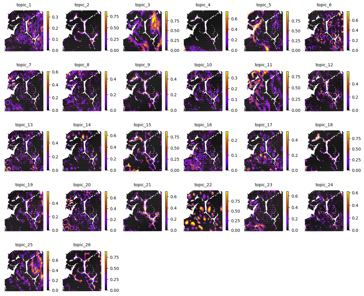
To visualize topic-spot distribution, use the mtopic.pl.topics function to generate scatter plots where each cell or spot is colored according to the proportion of a selected topic. This reveals spatial patterns and gradients that help interpret biological variation within the tissue.

mtopic.pl.topics(mdata, x="coords")

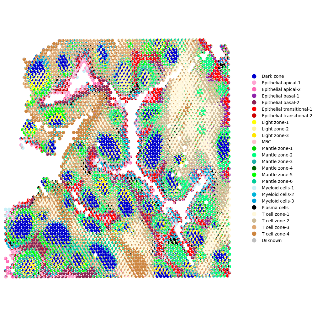
To visualize overall trends in topic distributions, use the mtopic.pl.scatter_pie function. This function visualizes the complete topic composition of each cell or spot as a pie chart.

The resulting plot provides a global overview of topic proportions across the tissue, helping you quickly identify regions enriched in specific topics. These regions may correspond to distinct cell types, tissue structures, or gradients of biological activity.

This visualization is handy for detecting the tissue’s spatial domains and functional zones.

Below, we apply the color palette (mdata.uns["TOPIC_COLOR"]) and cell type annotations (mdata.uns["TOPIC_CELLTYPE"]) prepared earlier for each topic.

mtopic.pl.scatter_pie(mdata,
                      x="coords",
                      radius=0.0073,
                      palette=mdata.uns["TOPIC_COLOR"],
                      annotation=mdata.uns["TOPIC_CELLTYPE"])

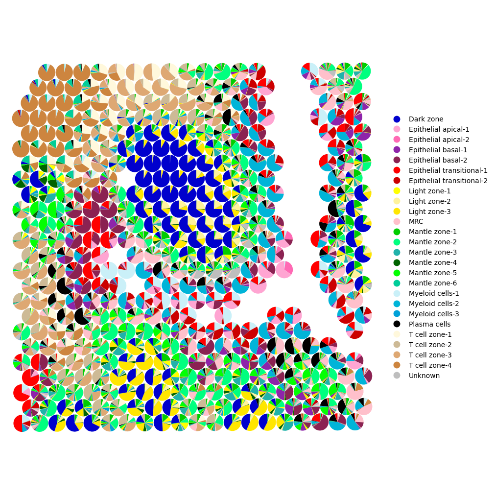
To focus on a specific region, you can limit the number of visualized spots using the xrange and yrange parameters (default value plotting all spots: [0, 1]), which define the fraction of the spatial extent to display.

mtopic.pl.scatter_pie(mdata,
                      x="coords",
                      radius=0.0073,
                      palette=mdata.uns["TOPIC_COLOR"],
                      annotation=mdata.uns["TOPIC_CELLTYPE"],
                      xrange=[0.3, 0.6],
                      yrange=[0.35, 0.65])

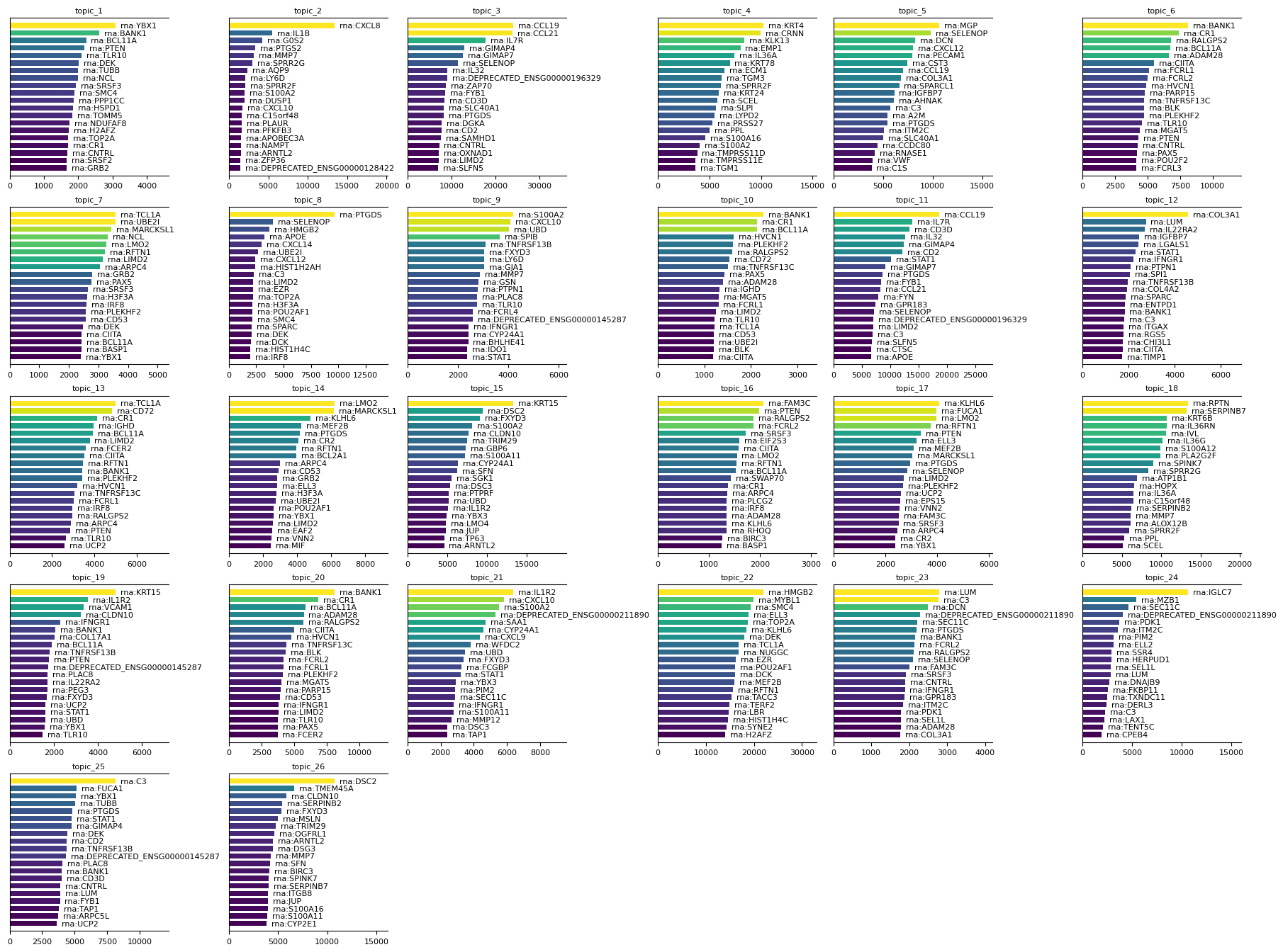
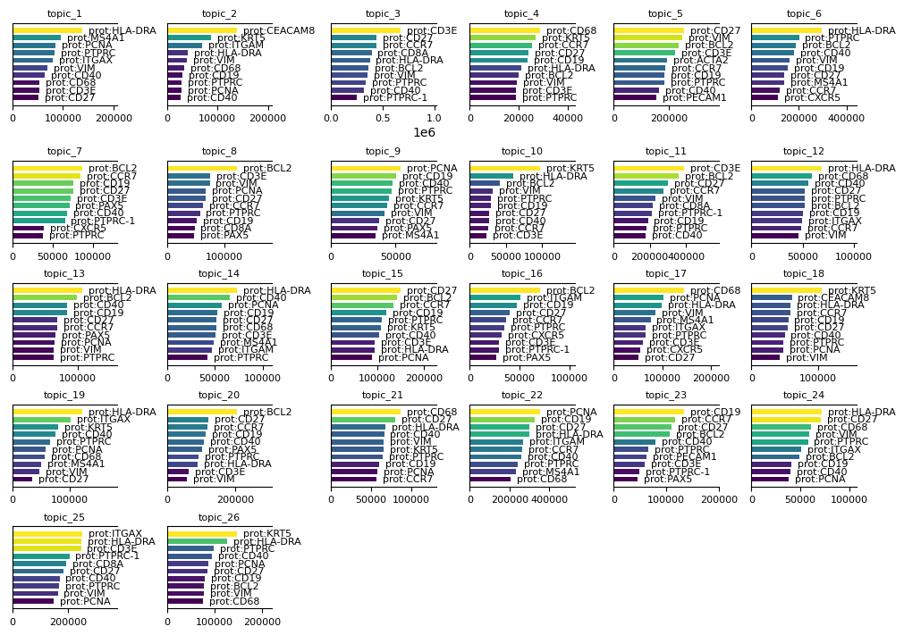
To interpret the results of the sMTM model, it is important to examine the feature signatures associated with each topic. Use the mtopic.pl.signatures function to visualize the top features per topic. These visualizations help reveal which molecular markers distinguish topics, aiding in biological interpretation and annotation of the results.

mtopic.pl.signatures(mdata, mod="rna", n_top=20)

mtopic.pl.signatures(mdata, mod="prot", n_top=10, figsize=(10, 7))

This concludes the application of mTopic for modeling spatial multimodal single-cell data, demonstrated using the human tonsil dataset.

mdata.write("HumanTonsil_trained.h5mu")