Tutorial 2: Spatial P22 Mouse Brain (ATAC + RNA)#

Welcome to tutorial on using the mTopic package for spatial multimodal topic modeling of the P22 mouse brain dataset with ATAC and RNA modalities.

In this tutorial, we will walk through the following steps:

scaling and normalizing the data,
applying spatial multimodal topic modeling to identify distinct cell populations and explore their functional roles,
visualizing the results to gain insight into the spatial distribution of topics and cell types within the tissue.

Let us begin by downloading the filtered training data, available at Zenodo.

[1]:

! wget -O P22MouseBrainATAC_filtered.h5mu \
  "https://zenodo.org/records/20044694/files/P22MouseBrainATAC_filtered.h5mu?download=1"

--2026-05-06 21:22:09--  https://zenodo.org/records/20044694/files/P22MouseBrainATAC_filtered.h5mu?download=1
Resolving zenodo.org (zenodo.org)... 137.138.153.219, 188.184.98.114, 188.185.43.153, ...
Connecting to zenodo.org (zenodo.org)|137.138.153.219|:443... connected.
HTTP request sent, awaiting response... 200 OK
Length: 42827881 (41M) [application/octet-stream]
Saving to: ‘P22MouseBrainATAC_filtered.h5mu’

P22MouseBrainATAC_f 100%[===================>]  40.84M  38.0MB/s    in 1.1s

2026-05-06 21:22:10 (38.0 MB/s) - ‘P22MouseBrainATAC_filtered.h5mu’ saved [42827881/42827881]

Spatial Multimodal Topic Modeling#

Load the prefiltered MuData object containing the dataset. This dataset includes 9,215 spatial spots and two modalities:

atac: chromatin accessibility data (50,000 peaks),
rna: gene expression data (10,000 genes).

[2]:

import mtopic

mdata = mtopic.read.h5mu("P22MouseBrainATAC_filtered.h5mu")

mdata

[2]:

MuData object with n_obs × n_vars = 9215 × 60000
  uns:      'CELLTYPE_COLOR', 'TOPIC_CELLTYPE', 'TOPIC_COLOR'
  obsm:     'coords'
  2 modalities
    rna:    9215 x 10000
    atac:   9215 x 50000

Before training the spatial Multimodal Topic Model (mtopic.tl.sMTM), it is essential to preprocess the data to improve the model’s ability to identify meaningful patterns across modalities.

To ensure comparability between ATAC and RNA data, we apply the following normalization and scaling steps:

TF-IDF transformation of ATAC and RNA (mtopic.pp.tfidf):

Adjusts raw counts by balancing feature frequency and importance, emphasizing rare but informative peaks/genes.
Scaling across modalities (mtopic.pp.scale_counts):

Linearly scales counts to ensure all modalities contribute equally during topic modeling, preventing one from dominating the analysis.

[3]:

mtopic.pp.tfidf(mdata, mod="atac")
mtopic.pp.tfidf(mdata, mod="rna")
mtopic.pp.scale_counts(mdata)

Now that the data is preprocessed, we can train the spatial Multimodal Topic Model (sMTM). This model identifies coordinated patterns (topics) across modalities while incorporating spatial information. It captures co-expression of peaks and genes, revealing distinct cell populations and their functional states. The training procedure comprises three steps:

Initialize the model:

Create an instance of the mtopic.tl.sMTM class, specifying the number of topics (n_topics) and other parameters. We use 50 topics for this tutorial.
Train the model:

Fit the model using variational inference (VI). This iterative process updates the model parameters to explain the observed data. While training time depends on dataset size, sMTM is optimized for scalability. While we use 500 iterations in this tutorial for thorough training, the model often converges to meaningful topics in as few as 20 iterations. You can adjust the number of iterations based on dataset size and desired precision.
Export trained parameters: Move inferred variational parameters to the MuData object.

[4]:

model = mtopic.tl.sMTM(mdata, n_topics=50, radius=0.06, n_jobs=100)
model.VI(n_iter=500)
mtopic.tl.export_params(model, mdata)

mdata

100%|██████████| 500/500 [1:09:32<00:00,  8.34s/it]

[4]:

MuData object with n_obs × n_vars = 9215 × 60000
  uns:      'CELLTYPE_COLOR', 'TOPIC_CELLTYPE', 'TOPIC_COLOR'
  obsm:     'coords', 'topics'
  2 modalities
    rna:    9215 x 10000
      varm: 'signatures'
      layers:       'counts'
    atac:   9215 x 50000
      varm: 'signatures'
      layers:       'counts'

Two families of variational parameters are produced during training.

First, topic distributions (variational parameters gamma) are stored in mdata.obsm["topics"] as a pandas.DataFrame of shape (n_obs, n_topics). Each row corresponds to a spatial spot or single cell and contains the topic proportions for that observation. These proportions sum to one for each spot and indicate the relative contribution of each topic to the molecular profile of the cell or spot. In spatial datasets, they can be interpreted as describing which biological programs are active in different tissue regions.

[5]:

mdata.obsm["topics"]

[5]:

	topic_1	topic_2	topic_3	topic_4	topic_5	topic_6	topic_7	topic_8	topic_9	topic_10	...	topic_41	topic_42	topic_43	topic_44	topic_45	topic_46	topic_47	topic_48	topic_49	topic_50
CTAAGGTCTTGCTGGA	0.000002	2.296221e-06	2.278458e-06	0.000002	2.759470e-06	2.280052e-06	2.280915e-06	2.304241e-06	0.000002	0.047534	...	8.559543e-02	2.313204e-06	2.327312e-06	2.293463e-06	0.000002	2.302036e-06	2.289454e-06	2.285268e-06	0.624707	2.290449e-06
CTAAGGTCACACAGAA	0.080414	4.195659e-06	4.156608e-06	0.000004	4.161522e-06	4.215305e-06	4.178711e-06	4.177182e-06	0.000004	0.025511	...	4.173739e-06	4.171695e-06	4.158175e-06	4.151908e-06	0.006123	4.141239e-06	4.162463e-06	4.174993e-06	0.000004	4.146406e-06
CTAAGGTCACAGCAGA	0.000003	3.119460e-06	3.097141e-06	0.149950	3.111266e-06	3.124094e-06	3.125135e-06	3.137151e-06	0.000003	0.000003	...	3.163105e-06	9.721310e-04	4.176197e-02	3.096804e-06	0.000003	3.099963e-06	3.110004e-06	3.135975e-06	0.298962	3.137222e-06
CTAAGGTCACCTCCAA	0.000003	3.294732e-06	3.247063e-06	0.000003	3.255979e-06	3.284710e-06	3.271618e-06	3.264278e-06	0.000003	0.000003	...	5.510247e-02	3.284523e-06	9.877103e-04	3.253502e-06	0.000004	3.247693e-06	3.255836e-06	3.285027e-06	0.000003	3.248571e-06
CTAAGGTCACGCTCGA	0.038988	9.233228e-07	2.030487e-02	0.000109	9.165386e-07	9.128643e-07	3.998651e-04	9.173582e-07	0.006390	0.008120	...	2.079242e-04	9.201721e-07	9.136634e-07	9.191915e-07	0.188788	9.138239e-07	9.138013e-07	9.199509e-07	0.087776	9.136199e-07
...	...	...	...	...	...	...	...	...	...	...	...	...	...	...	...	...	...	...	...	...	...
GAACAGGCGATGAATC	0.000001	1.314273e-06	1.305680e-06	0.000006	1.305992e-06	1.307464e-06	1.399463e-02	1.322107e-06	0.000001	0.000001	...	1.312560e-06	1.328176e-06	1.324196e-06	1.310480e-06	0.000001	1.322570e-06	1.310128e-06	1.319842e-06	0.790878	9.779936e-03
GAACAGGCGCCAAGAC	0.000001	1.061069e-06	1.041558e-06	0.000001	1.025889e-06	1.025753e-06	1.031231e-06	1.031470e-06	0.000001	0.000001	...	1.026589e-06	1.029366e-06	1.034609e-06	1.053661e-06	0.000001	1.029360e-06	1.057482e-06	1.039128e-06	0.000001	1.028081e-06
GAACAGGCCGGAAGAA	0.002539	1.024097e-02	4.906772e-07	0.000263	4.922969e-07	4.912472e-07	4.915815e-07	4.411158e-03	0.010943	0.002976	...	4.929855e-07	1.236522e-03	4.974992e-07	4.924651e-07	0.000274	6.900388e-03	4.919052e-07	4.925965e-07	0.905747	4.936819e-07
GAACAGGCGTGACAAG	0.000003	4.860141e-02	2.777212e-06	0.000474	2.803874e-06	2.774744e-06	2.781287e-06	6.588975e-02	0.000003	0.000003	...	2.795514e-06	1.761377e-02	4.483745e-02	8.287831e-02	0.000003	2.817490e-06	2.792463e-06	2.789886e-06	0.383127	2.789383e-06
GAACAGGCGAACCAGA	0.000002	7.527847e-03	2.397172e-06	0.160029	2.447559e-06	2.392231e-06	2.401329e-06	2.421732e-06	0.000002	0.183101	...	2.430198e-06	8.481727e-04	2.438826e-06	2.400039e-06	0.000003	2.431715e-06	2.414944e-06	2.406458e-06	0.212255	2.401081e-06

9215 rows × 50 columns

Second, modality-specific feature signatures (variational parameters lambda) are stored in mdata.mod[modality_name].varm["signatures"] as a pandas.DataFrame of shape (n_features, n_topics). Each column corresponds to a topic and represents the distribution over features within that modality. The values quantify the contribution of each feature (e.g., genes in RNA or peaks in ATAC) to the corresponding topic. Sorting features by their weights within a topic yields a ranked list of features that defines the characteristic signature of that topic for the given modality.

[6]:

mdata.mod["rna"].varm["signatures"]

[6]:

	topic_1	topic_2	topic_3	topic_4	topic_5	topic_6	topic_7	topic_8	topic_9	topic_10	...	topic_41	topic_42	topic_43	topic_44	topic_45	topic_46	topic_47	topic_48	topic_49	topic_50
Ppp1r14c	243.316012	0.010000	0.010000	429.106085	26.193395	0.010000	164.760756	255.891004	0.010000	1805.827246	...	279.341296	0.010000	169.725150	55.493814	1226.227057	96.826560	0.010000	299.786457	361.558199	27.278885
Plekhg1	0.010000	133.736447	0.010000	36.009355	98.395148	85.719898	22.148666	55.415516	31.481249	939.776390	...	99.871695	114.365941	534.057858	77.035102	156.449431	0.010000	77.841259	47.454673	718.468688	104.167555
Mthfd1l	35.621754	73.930607	79.105562	0.010000	103.597454	0.010000	0.010000	0.010000	36.180531	488.868888	...	85.114386	0.010000	185.505386	0.010000	121.937747	36.138333	32.310012	0.010000	329.355340	118.486533
Ccdc170	0.010000	0.010000	0.010000	0.010000	0.010000	0.010000	0.010000	0.010000	0.010000	0.010000	...	0.010000	0.010000	0.010000	0.010000	0.010000	44.293401	0.010000	0.010000	0.010000	0.010000
Esr1	0.010000	0.010000	0.010000	0.010000	0.010000	0.010000	0.010000	0.010000	0.010000	0.010000	...	47.517758	0.010000	0.010000	53.901852	0.010000	0.010000	0.010000	38.323073	203.831400	41.056238
...	...	...	...	...	...	...	...	...	...	...	...	...	...	...	...	...	...	...	...	...	...
Gm21722	0.010000	0.010000	0.010000	0.010000	0.010000	0.010000	0.010000	0.010000	0.010000	0.010000	...	0.010000	0.010000	0.010000	0.010000	44.231703	0.010000	0.010000	0.010000	0.010000	0.010000
Gm21857	0.010000	0.010000	0.010000	0.010000	0.010000	0.010000	0.010000	0.010000	34.638555	0.010000	...	0.010000	0.010000	0.010000	0.010000	0.010000	0.010000	0.010000	0.010000	0.010000	0.010000
Erdr1	132.012823	81.191155	152.639554	1384.061685	43.906190	371.252378	193.885278	104.761867	0.010000	2395.459744	...	374.282422	21.320315	1068.118309	70.898669	803.518433	47.106110	223.833447	0.010000	437.576037	125.193704
Gm21748	0.010000	0.010000	0.010000	0.010000	0.010000	0.010000	0.010000	39.435129	0.010000	0.010000	...	0.010000	0.010000	0.010000	0.010000	0.010000	0.010000	0.010000	0.010000	0.010000	0.010000
Gm21742	0.010000	0.010000	0.010000	0.010000	0.010000	0.010000	0.010000	0.010000	0.010000	0.010000	...	0.010000	0.010000	0.010000	0.010000	0.010000	0.010000	0.010000	0.010000	0.010000	0.010000

10000 rows × 50 columns

By preprocessing the data, training the sMTM model, and exporting the learned parameters, we have set the stage for the analysis of heterogeneity within the tissue.

Visualizing Topic-Spot Distribution#

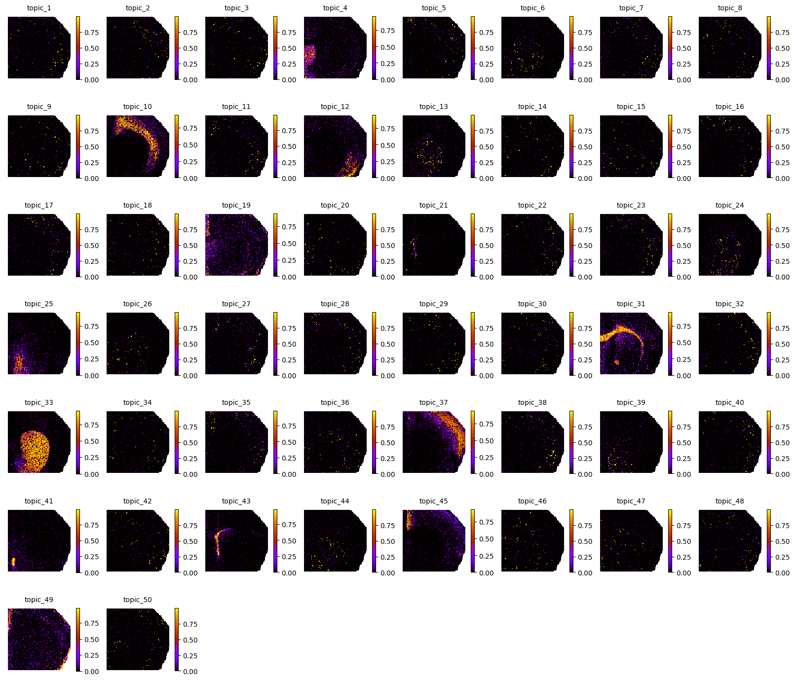
Visualizing topic distribution across cells or spatial spots is key in interpreting topic modeling results. This distribution reflects the contribution of each topic to each cell. They can reveal spatially organized cell states, types, or biological processes.

To visualize topic-spot distribution, use the mtopic.pl.topics function to generate scatter plots where each cell or spot is colored according to the probability of the selected topic. This reveals spatial patterns and gradients that help interpret biological variation within the tissue.

For example, if a topic captures a specific cell type, the plot will highlight regions enriched in that population.

[7]:

mtopic.pl.topics(mdata, x="coords", s=0.9, marker="s")

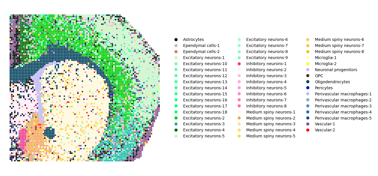
../_images/notebooks_T2_P22_Mouse_Brain_training_13_0.png

To visualize overall trends in topic-spot distributions, use the mtopic.pl.dominant_topics function. This function assigns each spot to its most dominant topic, the one with the highest probability, and colors it accordingly.

The resulting plot provides a global overview of topic dominance across the tissue, helping you quickly identify regions enriched in specific topics. These regions may correspond to distinct cell types, tissue structures, or gradients of biological activity.

This visualization is handy for detecting the tissue’s spatial domains and functional zones.

Below, we apply the color palette (mdata.uns["TOPIC_COLOR"]) and cell type annotations (mdata.uns["TOPIC_CELLTYPE"]) prepared earlier for each topic.

[8]:

mtopic.pl.dominant_topics(mdata,
                          x='coords',
                          s=60,
                          figsize=(13, 6),
                          palette=mdata.uns["TOPIC_COLOR"],
                          annotation=mdata.uns["TOPIC_CELLTYPE"],
                          legend_ncol=3,
                          markerscale=2)

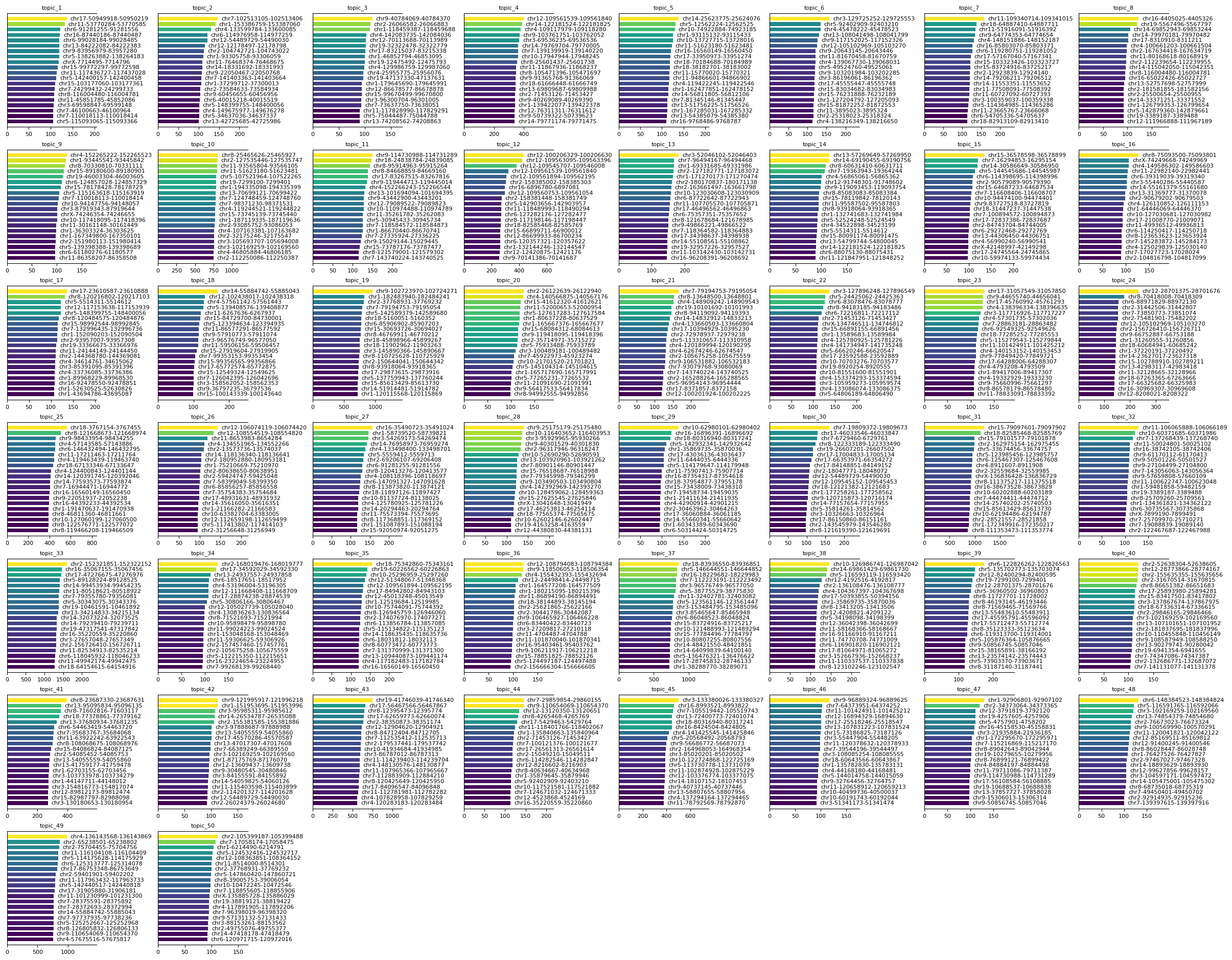
../_images/notebooks_T2_P22_Mouse_Brain_training_15_0.png

Visualizing Feature Signatures#

To interpret the results of the sMTM model, it is important to examine the feature signatures associated with each topic. Identifying the most relevant features for each topic provides insight into the biological identity and function of the inferred cell populations or processes.

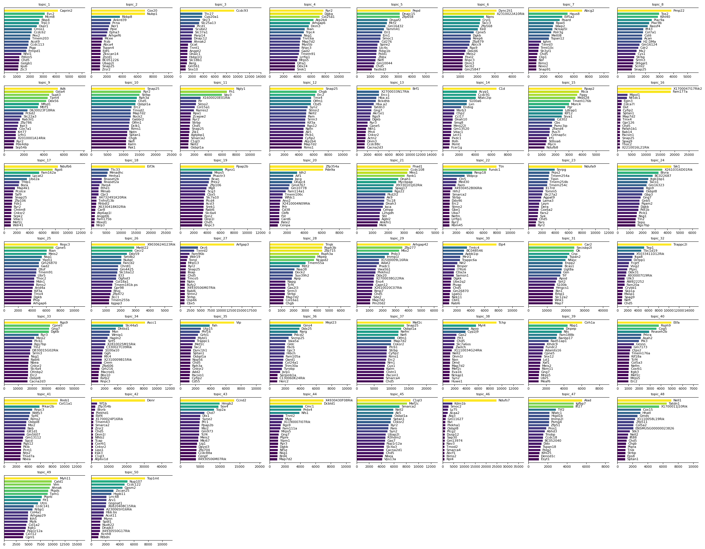
Use the mtopic.pl.signatures function to visualize the top features per topic. This function generates a set of plots, each showing the most significant features ranked by their scores for a given topic.

These visualizations help reveal which molecular markers distinguish topics, aiding in biological interpretation and annotation of the results.

[9]:

mtopic.pl.signatures(mdata, mod="atac", n_top=20)

../_images/notebooks_T2_P22_Mouse_Brain_training_17_0.png

[10]:

mtopic.pl.signatures(mdata, mod="rna", n_top=20)

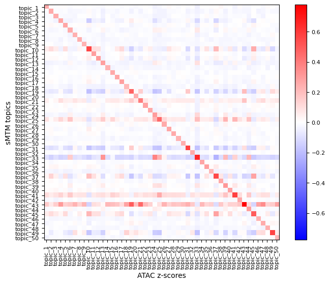
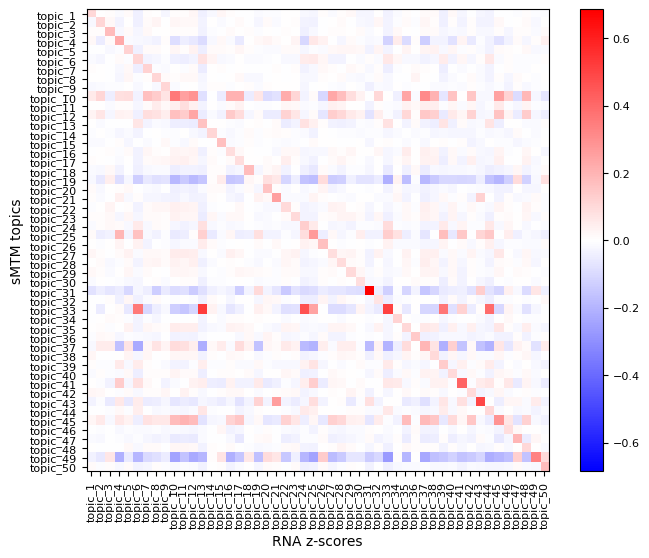
../_images/notebooks_T2_P22_Mouse_Brain_training_18_0.png

To better understand the spatial relevance of topic signatures and validate their biological specificity, you can visualize feature z-scores. A z-score indicates how much a feature’s expression in a given cell deviates from the mean, normalized by standard deviation. This highlights significantly up- or downregulated features in specific regions or cell populations.

Use mtopic.tl.zscores to compute modality-specific z-scores, and mtopic.pl.corr_heatmap to visualize their correlation with topic-spot distributions.

In the example below, we compute z-scores for the top 100 peaks and top 20 genes per topic to explore their spatial expression patterns.

[11]:

mtopic.tl.zscores(mdata,
                  raw_data_path="P22MouseBrainATAC_filtered.h5mu",
                  mod="atac",
                  n_top=100)

mtopic.pl.corr_heatmap(arr1=mdata.obsm["topics"],
                       label1="sMTM topics",
                       arr2=mdata.mod["atac"].obsm["zscores"],
                       label2="ATAC z-scores")

../_images/notebooks_T2_P22_Mouse_Brain_training_20_0.png

[12]:

mtopic.tl.zscores(mdata,
                  raw_data_path="P22MouseBrainATAC_filtered.h5mu",
                  mod="rna",
                  n_top=20)

mtopic.pl.corr_heatmap(arr1=mdata.obsm["topics"],
                       label1="sMTM topics",
                       arr2=mdata.mod["rna"].obsm["zscores"],
                       label2="RNA z-scores")

../_images/notebooks_T2_P22_Mouse_Brain_training_21_0.png

This concludes the application of mTopic for modeling spatial multimodal single-cell data, demonstrated using the P22 mouse brain dataset. We have walked through preprocessing, topic modeling, and result interpretation, highlighting how mTopic enables a joint analysis across modalities with spatial context.

[13]:

mdata.write("P22MouseBrainATAC_trained.h5mu")

Tutorial 2: Spatial P22 Mouse Brain (ATAC + RNA)

Contents

Tutorial 2: Spatial P22 Mouse Brain (ATAC + RNA)#

Spatial Multimodal Topic Modeling#

Visualizing Topic-Spot Distribution#

Visualizing Feature Signatures#